 2016, Vol. 37

2.大连理工大学 电子信息与电气工程学部, 辽宁 大连 116024
2.Faculty of Electronic Information and Electrical Engineering, Dalian Unirersity of Technology, Dalian 116024, China
磁感应成像技术(magnetic induction tomography,MIT)是一种具有非接触性、非侵入性、可检测磁性材料等优点的电学层析成像技术[1, 2, 3],又称作电磁层析成像(electromagnetic tomography ,EMT).它通过给激励线圈加交变电流使之产生磁场,该磁场穿过被测物体,会在被测物体内产生感应涡流,该感应涡流又会产生感应磁场,即二次磁场,该二次磁场携带物体内部参数信息,在检测线圈上会检测到该磁场信号,并传给计算机系统[4].MIT非常适用于医疗应用,尤其对还未发生病变,但对存在潜在危险的癌症早期等疾病起到预防和治疗的作用.MIT图像重建即逆问题是MIT技术的重要组成部分,而MIT图像重建算法的好坏将直接影响到重建图像(电导率或磁导率分布)的质量.LBP和Landweber是目前现有的MIT图像重建算法.LBP算法优点是成像速度快,无需迭代,但是由于该算法理论基础不够完善,导致重构出的图像失真较大.Landweber方法是当前MIT图像重建中较普遍的一种迭代算法[5] ,由于其适应于大部分典型流型,且编程简单,比较容易实现.但由于迭代序列使其收敛速度比较慢且精度低,这就无法满足MIT系统在线实时观测的要求.
本文提出一种设置门限阈值的方法来加快其收敛速度,并为了适应于MIT系统,在每次迭代中都自适应地调节阈值参数,从而提高图像重建的质量,也加快了收敛速度.
1 MIT数学模型MIT技术本质是对时谐涡流场中的边值问题求解[6]:
通过有限元方法求式(1)的边值问题相当于求解极值的变分问题:
经离散化,变成求解节点矢量磁位值的矩阵方程[7]:
检测线圈上的感应电压为
灵敏度S是检测线圈电压值的变化与电导率的变化之比:
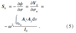
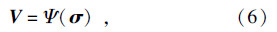
MIT正问题可表示成时谐涡流场问题,即电压V和电导率σ的关系:
则相应的逆问题为
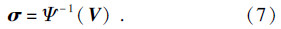
式(7)往往是欠定的且是非线性的.图 1展示了正逆问题的关系.

|
图1 正逆问题的关系 Fig. 1 Relationship between forward and inverse problem |
Landweber的基本思想[5]是最小化目标:

函数f(σ)对应的梯度为

根据梯度下降法,如果函数f(σ)在点σ=σk处有定义并且可微,那么函数f(σ)在σ=σk点沿着负梯度方向-∇f(σ)下降最快.基于此,为了求解式(8),可以提出以下迭代公式:

提高收敛速度的投影算子:
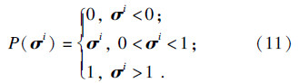
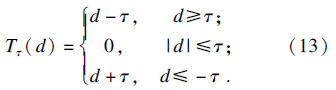
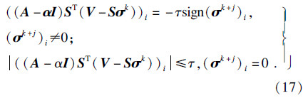
由于Landweber算法的收敛性较差,成像质量依赖于参数α的选择.通过设置门限阈值可以加快收敛速度[9].设定门限阈值,将很容易求解式(10),其形式为
让d=(σk+1)i,有
参数τ的选择非常重要,选择一个适应MIT系统的参数τ的思想是:如果让设置门限值后的结果约等于Landweber多步迭代后的结果,图像重建会很快收敛,这就导致

根据Landweber迭代算法,能得到多步迭代:
根据式(12)和式(13)可知:
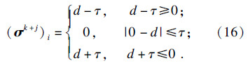
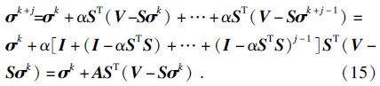
联合式(14)和式(15):
对于整个向量σk有

根据不同的A或j,能得到不同种类的最小值τ.通过实验可获得最优的A或j.
具体实现步骤:
步骤1 根据公式(15)计算矩阵A,根据公式(18)计算参数τ.
步骤2 以迭代的方式更新式(12)和(13).
步骤3 在每次迭代后,根据式(11)更新估计投影.
步骤4 迭代次数k在不断增加的同时,也不断重复步骤2.当式(6)达到足够小时,终止迭代过程. 步骤5 计算时间和误差.
3 仿真实验为了验证阈值Landweber算法的性能,本文利用Comsol Multiphysics仿真软件建立MIT系统的测量模型.表 1为LBP,Landweber和本文算法的重建图像.
| 表1 原始图和不同算法的图像重建结果 Table 1 Original figure and image reconstruction with different algorithms |


由表 1可知,本文算法(利用阈值Landweber算法)得出的图像边缘清晰,优于LBP和Landweber算法得出的图像重建效果.
由表 2可知,在同一种模型下,相同的迭代次数,本文算法的重建图像时间明显小于Landweber迭代算法.由于LBP无需迭代自然时间很短.
| 表2 不同算法的计算时间 Table 2 Computing time of different algorithmss |
图像重建误差是指重建图像与原始图像之间的相对误差:
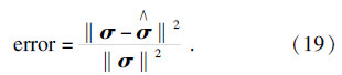
 为重建后电导率向量.
由表 3可知,本文算法的图像误差比LBP、未加阈值Landweber图像重建算法要好得多 .由此证明了本文算法的重建图像的视觉效果清晰、误差小.
| 表3 不同算法的相对误差 Table 3 Relative error of different algorithms |
本文在分析MIT系统基本理论的基础上,提出了一种阈值Landweber图像重建算法.通过仿真实验证明本文算法的图像效果和误差均比LBP,Landweber图像重建算法要好得多,且收敛速度快.由此可见,本文算法用于MIT图像重建有效且精度较高,值得进一步研究和推广.
| [1] | Griffith H.Magnetic induction tomography [J].Measurement Science and Technology, 2001,12(8):1126-1131.( 1) 1) |
| [2] | Wang J W,Wang X.Application of particle filtering algorithm in image reconstruction of EMT[J].Measurement Science and Technology, 2015,26(7):5303-5310.(1) |
| [3] | Merwa R,Hollaus K,Oszk B,et al.Detection of brain oedema using MIT:a feasibility study of the likely sensitivity and detectability [J].Physiological Measurement,2004,25(3) 347-354.(1) |
| [4] | Ma X,Peyton A J,Higson S R,et al.Hardware and software design for an electromagnetic induction tomography (EMT) system for high contrast metal process applications [J].Measurement Science and Technology,2006,17(6):111-118.(1) |
| [5] | Zhang M,Ma L,Soleimani M.Magnetic induction tomography guided electrical capacitance tomography imaging with grounded conductors[J]. Measurement,2014,53(7) :171-181.(2) |
| [6] | Hollaus K,Magele C,Merwa R,et al.Numerical simulation of the eddy current problem in magnetic induction tomography for biomedical applications by edge elements [J].IEEE Transaction on Magnetics,2004,40(3):623- 626.(1) |
| [7] | Soleimani M,Lionheart W R B,Peyton A J,et al.A three-dimensional inverse finite-element method applied to experimental eddy-current imaging data[J].IEEE Transaction on Magnetics,2006,42(10):1560-1567.(1) |
| [8] | Bertero M,Piana P.Projected Landweber method and preconditioning [J] .Inverse Problems, 1997,13(4):441-464.(1) |
| [9] | Daubechies I,Defrise M,Mol C D.An iterative thresholding algorithm for linear inverse problems with a sparsity constraint[J].Communications on Pure and Applied Mathematics, 2004,57(11):1413-1457.(1) |